Code the machine learning models
Now the machine learning models from Lesson 4: random forest, gradient boosting, and an LSTM. scikit-learn fits the first two in one line each. At the end you will draw a real forecast chart with matplotlib. Press Run on each block.
Step 1: build the features
Same as Lesson 4: three clues, each built only from days before the one we predict, then a time split into past (train) and future (test).
import pandas as pd

prices = [52.50, 57.15, 58.00, 60.00, 58.99, 58.95, 58.50, 60.00,
          61.00, 60.77, 61.00, 62.99, 62.98, 63.00, 65.00, 66.45,
          70.00, 74.95, 75.35, 74.50]
ncb = pd.DataFrame({"close": prices})

ncb["lag1"] = ncb["close"].shift(1)                 # yesterday
ncb["ma3"]  = ncb["close"].shift(1).rolling(3).mean() # 3-day average
ncb["mom"]  = ncb["close"].shift(1) - ncb["close"].shift(4) # momentum
data = ncb.dropna()

feat = ["lag1", "ma3", "mom"]
train, test = data.iloc[:11], data.iloc[11:]
print("train rows:", len(train), " test rows:", len(test))train rows: 11 test rows: 5
Models 1 and 2: random forest and gradient boosting
Both are tree models from scikit-learn, and both train in one line. We check each against the naive baseline on the test days.
from sklearn.ensemble import RandomForestRegressor, GradientBoostingRegressor
import numpy as np

rf = RandomForestRegressor(n_estimators=200, random_state=0).fit(train[feat], train["close"])
gb = GradientBoostingRegressor(random_state=0).fit(train[feat], train["close"])

for name, model in [("Random forest", rf), ("Gradient boosting", gb)]:
    mae = np.mean(np.abs(model.predict(test[feat]) - test["close"]))
    print(name, "test MAE: J$", round(mae, 2))

naive = np.mean(np.abs(test["close"].values[1:] - test["close"].values[:-1]))
print("Naive baseline test MAE: J$", round(naive, 2))Random forest test MAE: J$ 3.40 Gradient boosting test MAE: J$ 3.05 Naive baseline test MAE: J$ 2.24
On this short, strongly rising series the tree models actually trail the simple naive guess. Here is why: a tree can never predict a price higher than any it saw in training, so when the stock keeps climbing past its old range, the trees get stuck. With years of data and calmer stretches they shine, but this is a real reminder to always check the test error before trusting the shiny model.
Model 3: an LSTM neural network
The third model, an LSTM, is a neural network with a memory for sequences. It needs a deep-learning library like Keras and a lot more data to shine, so here is just the shape of it, to read rather than run.
from keras.models import Sequential
from keras.layers import LSTM, Dense

model = Sequential([
    LSTM(32, input_shape=(window, n_features)),
    Dense(1)                    # one number out: the next price
])
model.compile(optimizer="adam", loss="mae")
model.fit(X_train, y_train, epochs=50)
Draw the forecast with matplotlib
Numbers are one thing, a picture is another. matplotlib plots the model's forecast against the real prices in a few lines. Here we chart a simulated stock, AI Boss Inc, over its last 25 days. Press Run to see the figure.
import matplotlib.pyplot as plt

# aiboss: the last 25 test days of AI Boss Inc
plt.figure(figsize=(7, 3.5))
plt.plot(aiboss["day"], aiboss["actual"], label="Actual")
plt.plot(aiboss["day"], aiboss["pred"], "--", label="Model prediction")
plt.title("AI Boss Inc: model forecast vs actual")
plt.legend()
plt.show()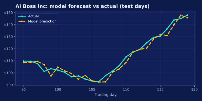
Outputs here are pre-generated so you can read along without a Python setup. On the real thing, that chart is the first thing an analyst looks at.
- Random forest and gradient boosting train in one scikit-learn line each.
- Tree models cannot predict beyond the prices they trained on, so check the test error first.
- An LSTM is a neural network for sequences; it needs Keras and lots of data.
- matplotlib draws a forecast-versus-actual chart in a handful of lines.
Last stop: the quiz, your certificate, and the live NCB challenge.